


Machine Learning for Turbulence Modelling
If you’ve studied turbulence and turbulence models you may have heard some of these phrases:
“When I meet God, I am going to ask him two questions: Why relativity? And why turbulence? I really believe he will have an answer for the first." -Werner Heisenberg
“Does Turbulence need God?” -William K. George
Questions regarding the nature of God and the origin of man aside, turbulence has puzzled our greatest minds for generations. Quite an unfortunate fact of life considering that much of the technology and devices we have deeply incorporated into our lifestyles deal with turbulent flow.
Since the advent of machine learning (ML), and more precisely the recent burst of interest in academia and industry in machine learning, there has been a reinvigorated thrust for innovation in the turbulence modelling community as well.

.gif)
Figure 1: Video of combustion with turbulence flow present.
Turbulence Modelling: Turbulent Flow
As the landscape of methodologies and tools continues to trend digital in industrial equipment design, manufacturing, and operation, the availability of useful data is further increasing. This, in addition to more accessible sophisticated machine learning algorithms, is a beautiful recipe for advancing the state-of-the-art in simulation.
Virtually all engineering applications are turbulent and hence require a turbulence model. Classes of turbulence models RANS-based models Linear eddy-viscosity models Algebraic models One and two-equation models Non-linear eddy viscosity models and algebraic stress models Reynolds stress transport models Large eddy simulations Detached eddy simulations and other hybrid models
This blog addressing turbulent flows serves to cover one of the most challenging aspects of Computational Fluid Dynamics (CFD) simulation (turbulence models and modelling), and frame it in the context of active research areas where machine learning is trying to help.
If all goes as intended, the blog will be approachable to those new to turbulence modelling and machine learning, while still being informative for turbulence model experts. Simcenter STAR-CCM+ and Monolith AI represent two software that fuse high-fidelity complex physics simulation and no-code machine learning software tailored towards engineering simulation.
Some founding and influential literature will be outlined in the table below to start. Then, some related topics will be explored in more detail. The first topic will be that of predicting the anisotropic nature of turbulence and turbulent flow, as well as the second on the scales of turbulence (with an example exemplifying how that may impact separation predictions).
These examples will strive to relate a sample of the machine learning predictions to their roots (spatially) in the Computational Fluid Dynamics (CFD) domain.
.png)
Figure 2: Some visualizations of the flow and turbulence in common canonical flow configurations
Literature Survey
The idea of step-reductions in simulation run time, or augmented accuracy in simulating turbulent flow, has the research and industry communities in a frenzy of excitement. Recently (summer 2021), professor Karthik Duraisamy (University of Michigan) hosted a symposium on model-consistent data-driven turbulence modelling [1]. Proceedings, agenda, and notes are provided by professor Duraisamy here (link).
There were sessions for: turbulence model consistency via field inversion, via integrated inference and learning, and also with evolutionary/symbolic techniques, among other things related to turbulent flow. Furthermore, important topics like benchmarking and emerging techniques were also covered. I highly recommend readers to review this wealth of knowledge from seminal leaders in the field.
Another exciting development in the turbulent model community is that from professor Weymouth (Southampton University). Also in the summer 2021, professor Weymouth published a model which uses deep learning based on the spanwise-averaged Navier–Stokes equations [2].
This Navier–Stokes equations approach strives to reduce the computational expense associated with the highly three-dimensional nature of turbulence through dimensionality reduction (averaging).
These spanwise-averaged equations contain closure terms that are modelled using a convolutional neural network. For the published use case, model predictions yield 90-92% correlation with the original 3-D system while taking only 0.5% of the CPU time.
In the image below, from top to bottom, the 3-D CFD solution is compared with the machine learning-based prediction as well as the 2-D CFD solution, respectively.
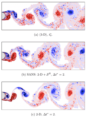
Figure 3: Comparisons of 3D, 2D, and machine learning predictions from Weymouth et al. [2]
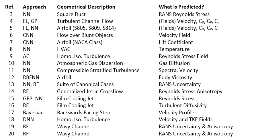
The table below presents a succinct list of studies that apply machine learning class methods to fluid flow mechanics problems, specifically, utilizing results generated from simulation-based investigations.
Some of the seminal works in this field are only recent to the last 5 years, making this a very exciting time for both the research community and industry.
Yarlanki from the IBM research group in 2012 was perhaps one of the earlier contributors on the relevant subject matter to the present turbulent flows article, whereby his study [8] conducted applied neural networks to an HVAC system, with the specific goal of predicting a temperature distribution.
While not taking a physics-informed approach in using the machine learning tool, there are many similarities in his approach to others that followed. Lauret [10] applied a neural network architecture to predict gas diffusion in an atmospheric fluid flow not long after in 2014.
In 2015, Julia Ling with the Sandia National Laboratories [13] published a major work that applied both neural networks and random forests to a suite of canonical problems. This is a major milestone when considering the research presented herein, on several accounts, and would go on to directly influence the directions taken in future studies [14, 15, 17, 17, 19].
First, it was among the first to apply both neural networks as well as random forest regression methods to CFD simulation data. Ling’s study showed that random forest methods, an extension of decision tree methods, have comparable accuracy to neural networks, and in fact provide their own unique advantages. One such advantage is the ability to acquire data from multiple sources, whereby each data set is not necessarily required to provide exactly the same features. This could allow for a data scientist to utilize one particular LES study which reported a set of features/results, and also utilize data from a separate LES study which only provided say 80% of the same variables, with some additional unique variables reported.
Another significant benefit analysing and predicting results with random forest regression methods is the ease of constructing the study to yield physically meaningful and interpretable results. Equivalently, this is termed physics informed machine learning, and allows for the machine learned predictions of fluid flow field variables to be interpreted with traditional engineering principles.
For example, some of Ling’s inputs (e.g. variations of vorticity) quantify the swirling and anisotropic nature of the fluid flow throughout the domain, with the algorithm’s predicted output being the uncertainty to expect from a RANS simulation. From basic CFD fundamentals, the limitations of RANS models are known, and do not counteract or conflict with the results from Ling’s machine learning results. This has clear value, as now the machine learning algorithms developed can be physically interpreted and regulated, as appropriate.
Several authors apply machine learning algorithms to canonical fluid flow configurations, such as turbulent channel flows, to study the nature of isotropic homogenous turbulence [4, 9, 18]. These studies target the Reynolds stresses as the output parameter to be learned and define a variety of input features to associate the relationship thereof.
The Reynolds stresses are a suitable choice, as they are one of the most transferable variables to quantify and describe the nature of the turbulence, and turbulent flows, amongst different unsteady flow configurations. These studies employ artificial neural networks, field (Bayesian) inversion, and autonomic closure methods.
Some studies [5, 7, 12] take a more applied approach, seeking to define the lift and drag on a variety of NACA shapes, to learn the relationship between airfoil shape and flow configuration to the output of these engineering quantifies. These studies apply field inversion techniques, convolutional neural networks, radial basis function neural networks, and traditional artificial neural networks.
The last category in this literature survey, summarized in the table, is that from the Stanford research group [16]. These works consider film cooling applications for machine learning methods, to improve computational fluid dynamics predictions. Specifically, the constitutive components and equations which are used to predict the turbulent flux of scalar values, embedded in the turbulence modeling framework (e.g. a basic gradient diffusion hypothesis, a constant value for turbulent Prandtl number throughout flow fields, turbulent diffusivity etc.).
While having little to do with the actual hydrodynamics, this is an important facet of the model, as the distribution of temperature in a film cooling environment is often the chief result of interest for a designer. In fact, previous Stanford investigations have shown that the concluded that the turbulent diffusivity definition was the single largest error source. To address this important concern, Milani [16] has constructed machine learning algorithms to predict the turbulent diffusivity throughout the flow field conducted on LES and DNS data sets, on film cooling jets and canonical cases (e.g. wall mounted cube).
Their results showed promise, as not only did the magnitude of the film effectiveness in the near-field injection from the machine learning predictions better approach the experimental ground truth data, but also the shape of the laterally averaged film effectiveness curves changed concavity to better match the experimental results.

Turbulence Modelling: Predicting Anisotropy in Turbulent Flows
Whether it be a property of a material, a temperature field, or an arbitrary characteristic of flow fields, the assumption of isotropy is seldom strictly correct. Often in engineering design work, the assumption of isotropy is used simply because there is no better option available. Turbulence and turbulent flows, unfortunately, is not an exception.
Considering disturbances in a fluid flow that generate turbulence (think of shearing), they are also often not isotropic. Even circumstances like grid-generated turbulence uniformly promotes turbulence quantities that would quickly become anisotropic if subject to acceleration downstream (e.g. grid generated turbulence upstream of an asymmetric nozzle).
This anisotropic quality of turbulence is quite cumbersome for eddy viscosity-based models to predict (and for turbulence models). Often, they take the approach to implicitly assume isotropic turbulence in their calculations for transport variables (turbulent kinetic energy); which from the preceding paragraph we now see as a departure from the truth.
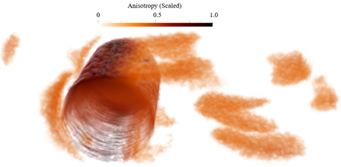
Figure 4: Cell groupings to depict the regions of the flow field (flow over a cylinder) which possess highly anisotropic turbulence
Recent interest has skyrocketed in applying machine learning-based approaches to learn the true nature of the anisotropy from higher fidelity simulations, such as Large Eddy Simulations (LES) which do not suffer from the same assumptions, and then somehow apply that knowledge back to lower fidelity eddy viscosity-based simulations.
Ling and Wang were great leaders in this research effort, publishing numerous seminal works [21, 22, 23] which evaluated how well machine-learning approaches could capture these distributions of anisotropy in flow fields.
Aids for visualization of the anisotropy, both as contours (right) and in Lumley triangles (left), can be seen below from Hodges [24]. For this domain of a film cooling jet, which is an applied variation of the classic jet in crossflow problem, scalar portrayal of an anisotropy ‘magnitude’ is shown as a contour within several wall normal planes. As the injected jet is deflected back towards the wall by the crossflow, the shearing between the streams indeed has higher levels of turbulence anisotropy, as well as near the wall where the gradients are highly anisotropic due to wall-blocking.
As such, these regions would be difficult for eddy viscosity-based models to predict. Bear in mind that eddy viscosity models show key regions influencing the resulting heat transfer at the wall and the aerodynamic performance; so quite important areas to get correct. The Lumley plots, with variations that are sometimes called Barycentric plots or turbulence triangles, strive to quantify whether the state of the turbulence model is highly one-, two-, or three-dimensional in nature. If three-dimensional, that is equivalently isotropic.
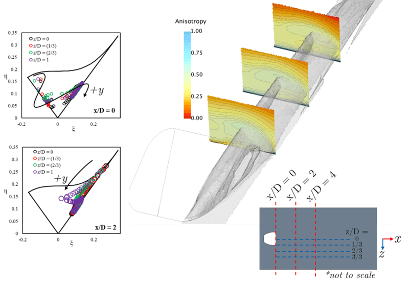
Figure 5: (Right) Scalar contours for the turbulence anisotropy in different planes for a film cooling jet flow field. (Left) Corresponding Lumley triangles which use data from boundary layer probes in each plane [24]
Now let’s pivot: aside from the possible value in improving our modelling approaches with machine learning, there is also possible value in better understanding the physics we are simulating with tools borrowed from machine learning and data science. You can also think about feature engineering, which is a typical step when creating a machine learning turbulence model.
For the example pictured above, the same simulation data can be processed with the popular t-stochastic distributed neighbor embedding (t-SNE) algorithm. In making a t-SNE plot, the outputs the machine learning model is trying to predict are represented by the handful of discrete colors used. The segregation, or clustering, of each color depends on how well the features selected can be correlated to said outputs.
For example- since we know smoking habits, dietary preference, and exercise patterns (these termed as the ‘inputs’) strongly correlate to cancer outcomes, a t-SNE plot showing the binary classification of cancer condition (yes- and no- each receiving their own respective colors, termed as the ‘outputs’) would result in strongly segregated and separated clusters for each color.
However, if we incorporated things we know are uncorrelated, such as favorite sports team, then the resulting plot and data clusters would be overlapping without clear zones of segregated colors in a given turbulence model.
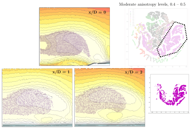
Figure 6: Based on Figure 5 data, a cluster from the t-SNE plot is segregated and mapped back into the CFD domain planes to reflect the location of such clusters in physical space.
Back to the film cooling flow example – in the above t-SNE plot we see each color represents a bin of anisotropy level (0-0.1, 0.1-0.2, …, 0.9-1.0). The grid points or inputs used were a large collection of fluid mechanics and turbulence parameters (e.g. turbulence intensity, wall-based Reynolds number, etc.).
For moderate levels of turbulent anisotropy, levels between 0.4 – 0.5 (shown in purple), one can see a relatively clear separation from the other levels. More interestingly, these points are lassoed with a dotted line are then mapped back into the wall-normal plains of the flow field. How fascinating – there is clear segregation! These points on the t-SNE map reside within the jetting fluid flow stream, enclosed between the mixing boundary layer with the freestream and the no-slip wall. Interestingly enough, it also excludes the center of the jet (potential core) in the first plane (x/D=0), which is less anisotropy due to being shielded from the shear velocity layers.
Additionally, this means that this physical region of the flow field is well posed for the machine learning model – that the ML turbulence model should be capable to provide an accurate ‘correlation’ between these sets of input features and the resulting anisotropy. How exciting!
Another classic problem, which is vital to many industries, is the flow over a cylinder (or bank of cylinders). A similar set of features are plotted in the mid-section of the flow domain. Some of the features may be familiar, such as turbulent viscosity ratio, while others are less so and more theoretical in nature (tensor invariants of strain rate tensor [25]).
While t-SNE may be a new concept to many readers, a contrast can be made to Principal Component Analysis. When comparing either plot generated from the same data, towards predicting the anisotropic nature of the turbulence, it is clear each has something unique to offer in regard to analysis and interpretability.
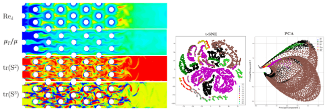
Figure 7: (Left) Different candidate features for a machine learning study plotted in the center plane of a pin fin bank flow field. (Right) Corresponding t-SNE and PCA representations of the same flow field based on turbulence anisotropy.
Setting Physical Scales for Turbulence kinetic energy
The largest scales contain most of the kinetic energy for the flow. As larger structures are broken into smaller ones, this energy is transferred to progressively smaller scales. The process of energy transfer from large to small scale is called direct energy cascade and it continues until the viscous dissipation can convert the kinetic energy into thermal energy. The scale at which this occurs is referred to as Kolmogorov length scale, after the mathematician Andrey Kolmogorov who worked on the energy cascade in turbulence.
Turbulence dissipation usually dominates over viscous dissipation everywhere, except for in the viscous sublayer close to solid walls. Here, the turbulence model has to continuously reduce the turbulence level, such as in low Reynolds number models. Or, new boundary conditions have to be computed using wall functions.
Perhaps one of the most coveted holy grails in turbulence modelling is the correct prediction of flow separation and reattachment. Regarding some of the most popular RANS models used in the industry for separated flow over the last decade, CFD practitioners have a very limited set of knobs to turn to responsibly calibrate their turbulence modelling for such models.
The transport equation for the turbulent dissipation rate equation, shown below, is one such destination that receives this attention for tweaking and tuning. One can speculate the origin of this is due to the fact that the turbulent kinetic energy equation, which has physical terms for production, destruction, and diffusion, while for turbulent dissipation there is no equivalently sensible form of turbulent kinetic energy.
The turbulent flow dissipation rate, and analogously the specific dissipation rate for the k-Ω based models, is how the timescale of the turbulence kinetic energy is determined. Whereas the turbulence kinetic energy sets the velocity scale.
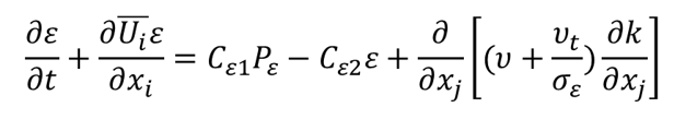
Of the many options available for customization and improvements, one example we can touch on is the Cε2 coefficient, which typically is a constant value simply determined by minimizing predictive error over a suite of canonical benchmark cases.
As shown in the pictures below for several different definitions for this coefficient, by changing this constant value to functions involving physical terms such as the anisotropy, one can significantly (and responsibly) vary the flow velocity field through this cylinder bank. Since these cases are under identical conditions otherwise, the separated flows, and separation patterns vary simply due to these different Cε2 definitions used.
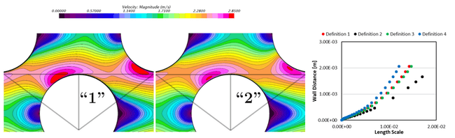
Figure 8: Resulting scalar fields (left) and boundary layer plots (right) for flow through a cylinder bank with various functional definitions for the Cε2 coefficient
Now, by incorporating machine learning, the possibilities continue to be enticing as we see (pictured below) that machine learning models (red) can predict anisotropy distributions in foreign numerical simulations that match that of the reference data (LES, blue).
For these two images, which are Barycentric plots, two separate wall-normal traverses are made through the domain to sample the state of the turbulence anisotropy. Again, where each corner represents one-, two-, or three-dimensional turbulence.
Now the puzzle is coming together – on one hand we can see tools in our toolbelt for modifying our separation predictions based on our physical understanding of the flow, and on the other hand we see ways to leverage high-fidelity data to train machine learning turbulence models which are extremely predictive for a wide breadth of cases.
This represents just one of the many possibilities for implementing machine learning to augment our existing ways of modeling turbulence and ultimately improving turbulence models.
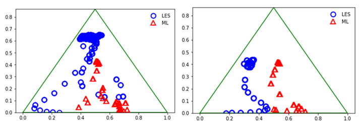
Figure 9: Turbulence triangle plots, for the anisotropy in a wall-normal profile, for LES data (blue, ground truth) and machine learning model predictions (red, attempting to replicate the LES data)
Additional Turbulent Flow Articles: Turbulence Modeling
Monolith AI and Simcenter STAR-CCM+ bring machine learning to CFD simulations, https://blogs.sw.siemens.com/simcenter/ai-for-cfd-simcenter/
4 Myths about AI in CFD, https://blogs.sw.siemens.com/simcenter/4-myths-about-ai-in-cfd/
Turbulent model References
[1] Duraisamy, K. (2021, July 27). Symposium on Model-Consistent Data-driven Turbulence Modeling. http://turbgate.engin.umich.edu/symposium/index21.html.
[2] Font, B., Weymouth, G. D., Nguyen, V. T., & Tutty, O. R. (2021). Deep learning of the spanwise-averaged Navier–Stokes equations. Journal of Computational Physics, 434, 110199.
[3] Cruz, Matheus Altomare. “MACHINE LEARNING TECHNIQUES FOR ACCURACY IMPROVEMENT OF RANS SIMULATIONS.“ Universidade Federal do Rio de Janeiro, 2018.
[4] Parish, Eric J., Karthik Duraisamy. “A paradigm for data-driven predictive modeling using field inversion and machine learning.“ Journal of Computational Physics, 305 (2016): 758-774.
[5] Singh, Anand Pratap, Shivaji Medida, Karthik Duraisamy. “Machine-learning-augmented predictive modeling of turbulent separated flows over airfoils.“ AIAA Journal, (2017): 2215-2227.
[6] Guo, Xiaoxiao, Wei Li, Francesco Iorio. “Convolutional neural networks for steady flow approximation.“ Proceedings of the 22nd ACM SIGKDD international conference on knowledge discovery and data mining, 2016.
[7] Zhang, Yao, Woong Je Sung, Dimitri N. Mavris. “Application of convolutional neural network to predict airfoil lift coefficient.“ 2018 AIAA/ASCE/AHS/ASC Structures, Structural Dynamics, and Materials Conference, 2018
[8] Yarlanki, S., Bipin Rajendran, and H. Hamann. “Estimation of turbulence closure coefficients for data centers using machine learning algorithms.“ 13th InterSociety Conference on Thermal and Thermomechanical Phenomena in Electronic Systems, IEEE, 2012.
[9] King, Ryan N., Peter E. Hamlington, Werner JA Dahm. “Autonomic closure for turbulence simulations.“ Physical Review, E 93.3 (2016): 031301.
[10] King, Ryan N., Peter E. Hamlington, Werner JA Dahm. “Autonomic closure for turbulence simulations. “ Physical Review E, 93.3 (2016): 031301.
[11] Maulik, Romit, Omer San. “A neural network approach for the blind deconvolution of turbulent flows.“ Journal of Fluid Mechanics, 831 (2017): 151-181.
[12] Zhang, Weiwei, et al. “Machine learning methods for turbulence modeling in subsonic flows over airfoils.“ arXiv preprint, arXiv:1806.05904 (2018).
[13] Ling, Julia, J. Templeton. “Evaluation of machine learning algorithms for prediction of regions of high Reynolds averaged Navier Stokes uncertainty.“ Physics of Fluids, 27.8 (2015): 085103.
[14] Ling, Julia, et al. “Uncertainty analysis and data-driven model advances for a jet-in-crossflow.“ Journal of Turbomachinery, 139.2 (2017).
[15] Weatheritt, Jack, et al. “A comparative study of contrasting machine learning frameworks applied to RANS modeling of jets in crossflow.“ ASME Turbo Expo 2017: Turbomachinery Technical Conference and Exposition, American Society of Mechanical Engineers Digital Collection, 2017.
[16] Milani, Pedro M., et al. “A machine learning approach for determining the turbulent diffusivity in film cooling flows.“ Journal of Turbomachinery, 140.2 (2018).
[17] Edeling, Wouter Nico, Gianluca Iaccarino, Paola Cinnella. “Data-free and data-driven RANS predictions with quantified uncertainty.“ Flow, Turbulence and Combustion, 100.3 (2018): 593-616.
[18] Beck, Andrea D., David G. Flad, Claus-Dieter Munz. “Deep neural networks for data-driven turbulence models.“ arXiv preprint, arXiv:1806.04482 (2018).
[19] Wang, Jian-Xun, Jin-Long Wu, Heng Xiao. “Physics-informed machine learning approach for reconstructing Reynolds stress modeling discrepancies based on DNS data.“ Physical Review Fluids, 2.3 (2017): 034603.
[20] Wu, Jin-Long, et al. “A priori assessment of prediction confidence for data-driven turbulence modeling.“ Flow, Turbulence and Combustion, 99.1 (2017): 25-46.
[21] Ling, Julia, Andrew Kurzawski, and Jeremy Templeton. "Reynolds averaged turbulence modelling using deep neural networks with embedded invariance." Journal of Fluid Mechanics 807 (2016): 155-166.
[22] Ling, Julia, et al. "Uncertainty analysis and data-driven model advances for a jet-in-crossflow." Journal of Turbomachinery 139.2 (2017): 021008.
[23] Wang, Jian-Xun, et al. "A comprehensive physics-informed machine learning framework for predictive turbulence modeling." arXiv preprint arXiv:1701.07102 (2017).
[24] Hodges, Justin, and Jayanta S. Kapat. "Topology and Physical Interpretation of Turbulence Model Behavior on an Array of Film Cooling Jets." Turbo Expo: Power for Land, Sea, and Air. Vol. 58646. American Society of Mechanical Engineers, 2019.
[25] S. Pope, Journal of Fluid Mechanics 72, 331 (1975).